Spreadsheets usually hold a wealth of information, but it can be difficult to see what’s important in them, such as key data points and trends. There are several ways to make data stand out visually in an Excel spreadsheet, but one of the simplest and most effective is to apply conditional formatting.
What is conditional formatting in Excel?
Conditional formatting is a feature used to make unique, important, or duplicate values stand out or to emphasize trends in a data set. As the name suggests, the feature allows you to format the cells and their data based on conditions you specify, which makes important information easy to see at a glance.
Some common examples:
- Formatting cells that meet specific criteria with a highlight color and/or font
- Applying different colors to different cells based on their values
- Applying color scales or gradients to visually represent cells’ values
Crucially, conditional formatting is dynamic, so it keeps up when your data set changes. For instance, if you create a conditional formatting rule that highlights cells with values over 100, and one of the cells in your set changes from 95 to 102, that cell will become highlighted.
In this article we’ll show you different ways to apply conditional formatting to your data sets. When using conditional formatting, the first option you have is to use preset conditions — formatting options that are built into Excel. We’ll go over some of the best preset conditions for formatting, and then cover how to create your own custom formatting rules.
 Shimon Brathwaite / IDG
Excel offers several built-in conditional formatting rules you can apply to your data. (Click image to enlarge it.)
We’ll demonstrate using Excel for Windows under a Microsoft 365 subscription. If you’re using a different version of Excel, you might not have the same interface and options, but the features should work more or less the same way.
Before we begin: How to clear conditional formatting
Throughout this story, we’ll use the same example data set, applying one type of formatting, then clearing it away before applying the next type of formatting. So before we begin, we’ll quickly go over how to clear conditional formatting from a data set.
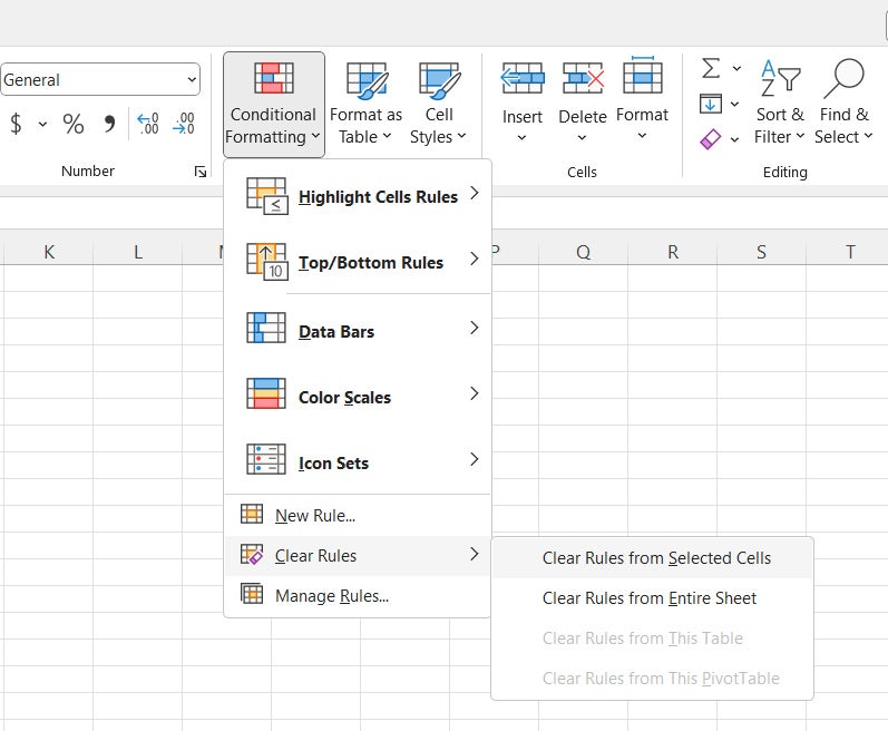
Simply navigate to the Excel Ribbon’s Home tab. Click the Conditional Formatting button and then select Clear Rules. There you can opt to clear conditional formatting from the selected cells, the entire worksheet, the current table, or the current PivotTable.
 Shimon Brathwaite / IDG
It’s easy to remove conditional formatting rules.
How to use highlight cells rules
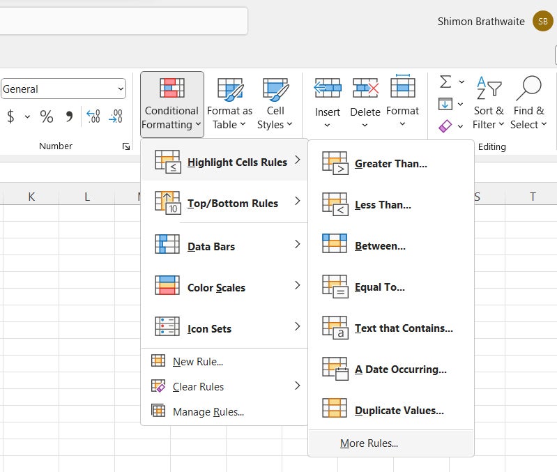
With that out of the way, we’re going to begin with highlight cells rules. These can be found on the Home tab under Conditional Formatting > Highlight Cells Rules.
 Shimon Brathwaite / IDG
The highlight cells rules options.
Here you can see multiple options for highlighting cells based on their values, including greater or less than a certain value, equal to a certain value, between certain values, containing certain text, with a certain date, with duplicate values, and more.
We’ll use the Greater Than option as an example. This will highlight any cells that are greater than a specified number within the data set. For example, you can choose to highlight all cells that are greater than the number 200.
Simply select the set of cells you want to format, then click on Home > Conditional Formatting > Highlight Cells Rules > Greater Than to open the following dialog box.
 Shimon Brathwaite / IDG
Filling out the conditions for a Greater Than formatting rule.
On the left, select the number to filter by. In this case we are going to highlight any number that is greater than 200. On the right, select the type of highlighting to apply or create a custom format.
As you can see from the screenshot below, the formatting is done in real time, so you can see the effects of your choice before you commit. To finalize your choice, click OK.
 Shimon Brathwaite / IDG
When you make a selection, the formatting is instantly applied to your data. (Click image to enlarge it.)
How to use top/bottom rules
Highlight cells rules are good when you have a specific value in mind, such as numbers greater than 100, cells containing specific words, and so on. But what happens if you need a relative measure — for example, you want to know the highest 10% of values in a data set? In that case, it’s best to use the Top/Bottom Rules option.
This option includes presets for the top or bottom 10 items in the data set, items in the top or bottom 10%, items above or below the average of the data set, and more. The top/bottom presets can be adjusted to show a different percentage or number of items.
Let’s see how these rules work using the Top 10% option. Once you have cleared the highlight cells rules from the data set, select the cells you want to apply the rule to, go to Home > Conditional Formatting > Top/Bottom Rules and select Top 10%.
 Shimon Brathwaite / IDG
Choosing a top/bottom rules preset.
Once you select that option, you will get a dialog box where you can adjust the exact top percentage you want to highlight and choose the style of the formatting.
 Shimon Brathwaite / IDG
Adjusting Top 10% conditions.
Once you have made your selections, hit OK to confirm the formatting.
Note that you can apply more than one set of conditional formatting rules to a data set — so you could, for instance, highlight the top 5 values in red and the bottom 5 values in yellow.
 Shimon Brathwaite / IDG
Our data set with the top 5 and bottom 5 values highlighted in different colors. (Click image to enlarge it.)
How to use data bars
Data bars show a visual representation of how a specific data point relates to the maximum value of the data set. For example, if the largest value in the dataset is 1,000, then a cell with a value of 500 would have a bar that is exactly 50% of the full width of the cell. This allows you to tell at a glance how large a value is compared to the maximum value.
 Shimon Brathwaite / IDG
Applying data bars formatting to a data set. (Click image to enlarge it.)
To set up data bars formatting, select the cells you want to apply the rule to, go to Home > Conditional Formatting > Data Bars, and choose one of the styles under Gradient Fill or Solid Fill.
How to use color scales
The color scales option highlights cells with different shades of color depending on how close they are to the data set’s maximum or minimum value. With the target cells selected, choose Home > Conditional Formatting > Color Scales.
 Shimon Brathwaite / IDG
Applying color scales formatting to a data set. (Click image to enlarge it.)
You can select any of the preset color scales provided, or you can select More Rules in order to change colors or add more colors for more customized data analysis. For example, if you choose a three-color scale, you can select any percentile you want to be represented by the third value. In the example shown here, I selected the 50th percentile.
 Shimon Brathwaite / IDG
Creating a custom color scale.
The final result is shown below.
 Shimon Brathwaite / IDG
Our custom color scale in action. (Click image to enlarge it.)
How to use icon sets
Finally, there are icon sets, which allow you to add icons such as arrows, shapes, flags, or stars to the cells that meet a predefined criterion. You can access this option via Home > Conditional Formatting > Icon Sets.
Select any of the icon sets shown, and it will rank each of the cells based on how close it is to the minimum and maximum number in the data set. For the example below, I selected the star icon set. The top value gets a yellow star and the midpoint a half-yellow star. Because all the other cells are in the bottom third by value, they get white stars.
 Shimon Brathwaite / IDG
Applying an icon set to the selected cells. (Click image to enlarge it.)
You can also use the More Rules option at the very bottom of the icon sets menu to customize the formatting to your liking.
 Shimon Brathwaite / IDG
Adjusting the value ranges for each icon.
How to create custom formatting rules
If none of these rules work for you, you may want to create fully custom rules from scratch. To do so, select the target cells, go to Home > Conditional Formatting > New Rule, and then select the appropriate rule type. In this case we will choose the second-to-last option, Format only unique or duplicate values, and then under “Format all:” in the “Edit the Rule Description” area, select duplicate.
 Shimon Brathwaite / IDG
When creating a custom formatting rule, first select the rule type, then edit its description below. (Click image to enlarge it.)
Once that is done, click the Format button. On the pane that appears, you can choose how you want to format the cells, including changing number layout, changing the font, changing the border, or filling the cell with a certain color. In this case we will select the Fill tab and choose the red fill color.
 Shimon Brathwaite / IDG
Choosing the styling for a custom formatting rule. (Click image to enlarge it.)
With the style selection made, click OK, and this style appears in the Preview area of the New Formatting Rule pane. Once you click OK or hit Enter, the cells with duplicate values are highlighted.
 Shimon Brathwaite / IDG
Only the cells with duplicate values are colored red.
Managing your conditional formatting rules
As mentioned previously, you can apply more than one conditional formatting rule to the same set of cells, and you can also have different formatting rules for different sets of cells in the same worksheet. To manage all these rules, go to Home > Conditional Formatting > Manage Rules. You’ll see a dialog box with your rules listed.
 Shimon Brathwaite / IDG
You can manage your rules in the Conditional Formatting Rules Manager. (Click image to enlarge it.)
To delete a rule, simply select it and click the Delete Rule button.
You can also create a new rule from this interface. Click the New Rule button, and you’ll be taken to the same New Formatting Rule dialog box covered in the previous section of the story.
To edit an existing rule, select it in the list and click the Edit Rule button. You’ll see the Edit Formatting Rule dialog box, where you can edit the formatting specifics of the currently selected rule. You can also change the cells the rule applies to by clicking the up arrow icon to the right of its “Applies to” box.
Before you edit a rule, it’s not a bad idea to create a copy of it. That way you’ll have a backup of the original rule that you can revert to if needed. To make a copy, select the rule and click Duplicate Rule.
A duplicate also comes in handy if you want to apply a rule to a different set of cells. You can duplicate the rule, then change the “Applies to” selection for the duplicate.
Copyright © 2023 IDG Communications, Inc.
This story originally appeared on Computerworld

